In the 1700s, Newton had shown that mixing two colors produces the sensation of a third color. By the twentieth century, it was already established that only three primary colors were needed to produce most other colors, and that three photoreceptor types (RGB, discussed in Chapter 2) were responsible for the human perception of color.
In the late 1920s, John Guild and William David Wright separately conducted similar experiments intended to measure color. In both experiments, observers were set up at a 2° field of view from a screen consisting of a “reference field” on one side and an “adjustment field” on the other side, as depicted below:
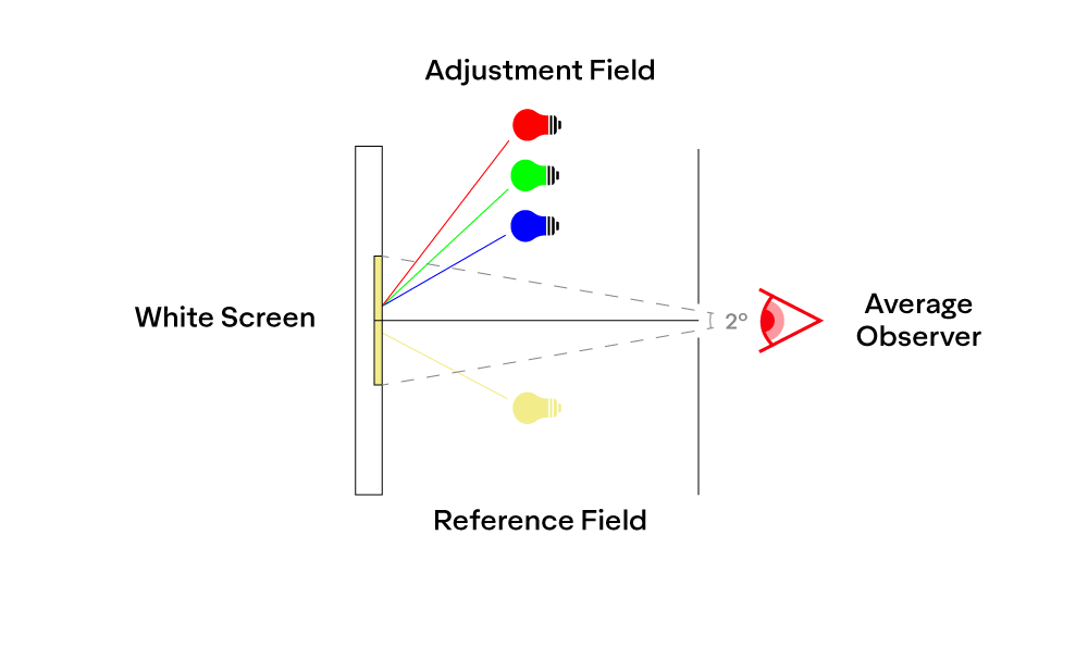 In the reference field, the experimenters would produce a color using a specific wavelength of light (monochromatic light). On the adjustment field the observers were asked to reproduce the color using a set of monochromatic red-, green-, and blue-colored lights.
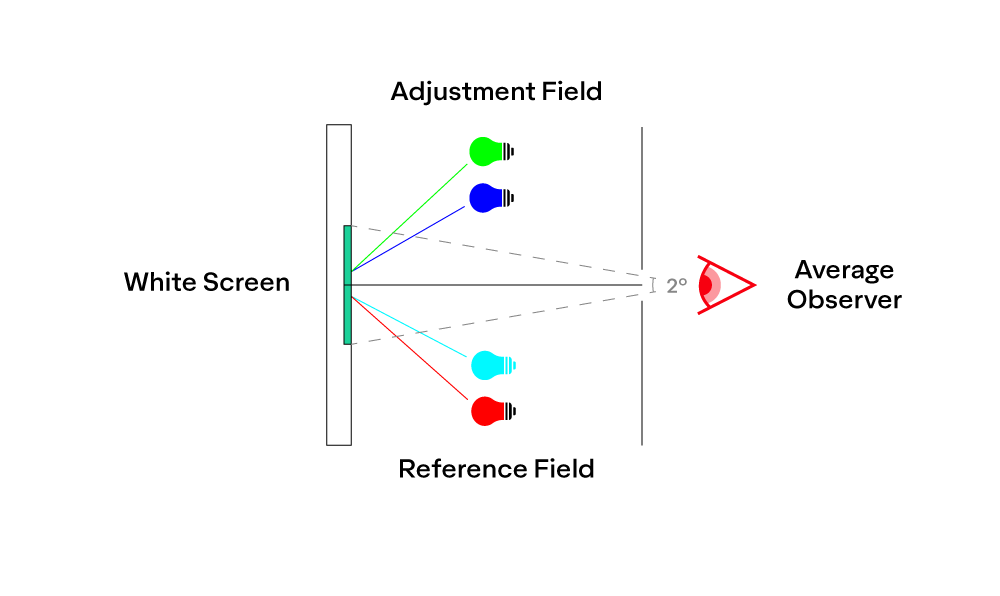
During these experiments, it was discovered that certain reference colors could not be matched by the three primary RGB colors. However, in the 1850s, Herman Grassman had shown that colors add together linearly; meaning that when two colors are mixed together, the resulting third color is somewhere in between the two initial colors, and if the intensity of the primary colors is known, the results could be expressed algebraically; this became known as Grassman’s law.
One implication of Grassman’s law is that colors can be mathematically calculated if there is a gap in between a set measured colors. So, to reproduce the colors that RGB alone could not, the subjects were asked to “subtract” a certain amount of red, green, or blue color from the reference side by mixing the same color into it. In other words, where they could not achieve a desired saturation of color on the adjustment side, they would desaturate the monochromatic light on the reference side.
For example, certain hues of cyan at about 500 nm on the reference field could not be visually matched by the observers on the adjustment field. To address this, observers were asked to instead add red to the adjustment field until both sides match:
 Each observer perceived color slightly differently, though the results were very similar. The results from the observers were averaged to produce the following Color Matching Function (CMF) for the “average observer”:
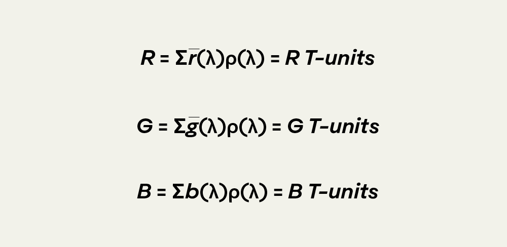
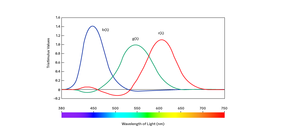 In the graph above, the x-axis represents the visible spectrum produced by the experimenters in the reference field of view, while the y-axis represents the relative intensity of the red, green, and blue lights used by the observers to reproduce the reference color in the adjustment field of view. Negative values represent desaturation of the reference color to achieve a match. The three R,G, and B values needed to match a certain color within the visible spectrum are known as the tristimulus values, typically referred to as “T-units”.
Knowing the relative intensity of each R, G, and B light to reproduce any colors along the visible spectrum in the 1920s, was a major breakthrough. Not only did it mean that RGB lights could be used to produce most colors, it meant that we can now quantify the appearance of any color by taking the spectral distribution (SPD) (Chapter 1), multiply it by the tristimulus values, and sum the results to get the relative intensity of each value:
Guild and Write presented their data to the International Commission on Illumination (CIE), which had been trying to standardize a way for labs and manufacturers around the world to measure color. After some back and forth (common with committee discussions) the commission began to manipulate the findings so that they could more easily be used in a standard.
To simplify the calculations, the tristimulus values were normalized by taking the individual values for each of the R, G, and B curve at each wavelength and dividing it by the sum of the R, G, and B value at the same wavelength:
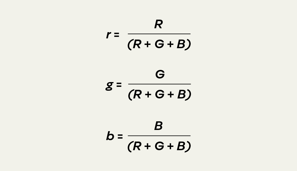
Normalizing the tristimulus values creates the following color matching function (CMF) and curves. Note that R,G, and B are now represented by lowercase, r, g, & b: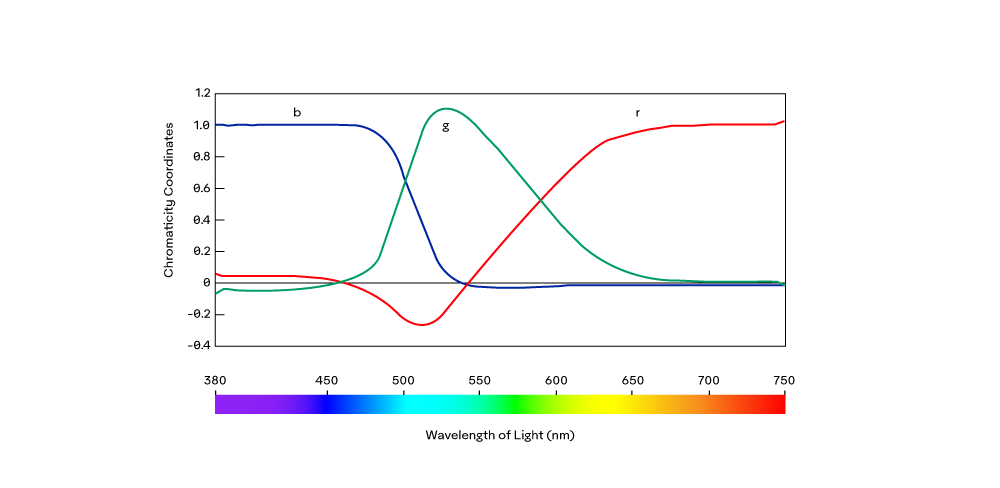
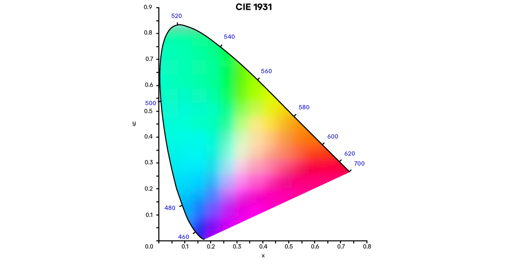
This was simpler because the sum of the r, g, and b values was now one, meaning that if we have two, we can derive the third. With this in mind, CIE then took the red and green values and plotted them against each other to create the following chromaticity “locus”:
.png)
Locus comes from the Latin word for place or location; essentially, it is the curve, shape, or as in this case, the “space” that is created when you connect data points. The locus (perimeter of the color space) in the above diagram represents spectral colors, while Grassman’s law was used to calculate the colors within the locus.
Examining the above diagram, there are a few items of note:
R, which represents the wavelength of a monochromatic red light, is where the red intensity is set to 1.0, and the green intensity is set to 0.0.
Conversely, G is located at red intensity 0.0 and green intensity 1.0.
If we select any two colors sufficiently apart from each other, mixing them would result in a third color along a straight line between the two initial colors.
Equal Energy white, or “EE white”, is located at red 0.333, green 0.333 (and blue 0.333 if it was not normalized out).
This new color space was a major step forward in standardizing color, but it still needed a few more refinements to be used in manufacturing worldwide. For instance, having negative numbers created a higher likelihood of mistakes in an age without personal computers. Additionally, negative numbers are generated with lights on the reference field, meaning that device manufacturers needed six channels of lights (3 in each field), as opposed to three.
Given the linear nature of color perception and the mathematical construction of the color space, CIE decided to use algebraic transformations to shift the color space into a positive quadrant. Additionally, the impact of brightness on color would be mathematically put into only one of the axes.
Using previous research from the eye's photopic response, discussed in Chapter 2, CIE knew the relative perceived luminance of the R, G, and B functions. The data was used to calculate new imaginary primaries that were not red, green, or blue but rather X, Y, and Z.
Further, CIE mathematically put all the luminance data into one of the primaries to simplify the rest. This resulted in the alychne, or the line of “no light”, shown below. We can see that the alychne starts at 0,0, and has a slope of -0.2/1.0. Meaning that there is no energy at 0,0, and as we move to the right, red is added, but a fraction of green is taken away (because we perceive green to be much brighter than red.) Likewise, as we go left from 0,0 and green is added, much more red is taken out. The result is that any measurement along the alychne would mathematically have zero luminance.
.png)
 From there, the straight line joining the R and G primaries was extended in both directions. Where the R & G line intersects, the alychne was labeled X. While Z and Y were established by a tangent line to the locus that also intersected the alychne and the R & G line. The alychne then replaced the red axis in the original r, g color space shown above. Finally, the algebraic transformation shifted everything so that the Y-Z line was perpendicular to the alychne. Because the imaginary primaries Z and X lay along the alychne, the Y primary carried all the luminance data.
The axes were re-labeled for simplicity and practicality but also to signify their mathematical nature. The red axis became the x-axis (small x because it still uses normalized data), and the green axis became the y-axis. Y, which carried the luminance data and was normalized to a perfectly white equal energy (EE) surface, became Y%, indicating how much luminance a color has compared to a perfectly white surface. The project ended in 1931 and became known as the CIE 1931 color space, which is still used to standardize color in manufacturing products today.